Peripheral Sensory Nerve Stimulation Selectivity Across Electrode Configurations and Placements

Objective and Hypothesis

Using extraneural cuff, interfascicular, and intrafascicular electrode placements, the project’s goal is to evaluate the selectivity and efficiency of peripheral sensory nerve stimulation with monopolar, bipolar, or tripolar configurations. Using COMSOL, an ulnar nerve model is used to compute voltage distributions for each of the nine conditions, and these results were analyzed in NEURON using the McIntyre–McNeal–Grill model to simulate peripheral nerve stimulation. We hypothesize that tripolar intrafascicular stimulation will yield the highest selectivity: the tripolar electrode placement will have two return electrodes that confine the current from neighboring fascicles, and the intrafascicular setup will have the electrode placed directly inside the fascicle to lower the amplitude required for an AP threshold (Becker et al., 2023). The goal is to inform future approaches that aim to selectively stimulate the sensory fascicle in the ulnar nerve for applications to functional electrical stimulation and sensory prostheses.

Methods: COMSOL Model

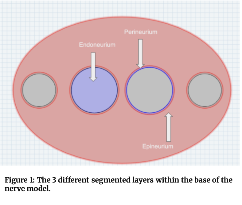
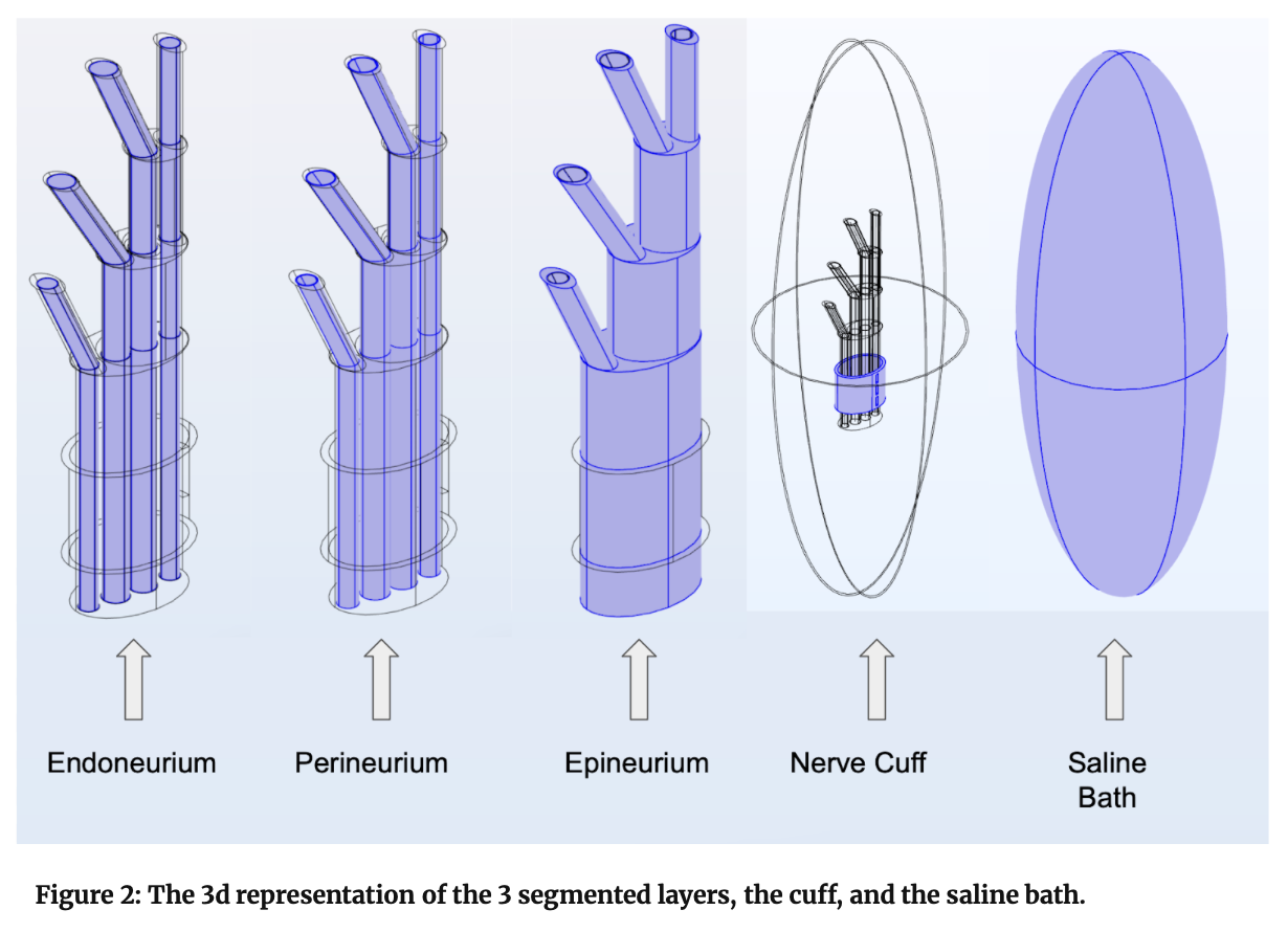
Our model began with a 2D base of the cross-sectioned ulnar nerve with four fascicles. The “difference” Boolean operator was used to segment the circles and ellipses representing the epineurium layer, the four perineurium layers, and the four endoneurium layers (Figure 1). The extrude function was later used to add a 3D representation of this base, serving as the nerve before the branch, which will be the target for stimulation. The nerve branching was then constructed using the same 2D-to-3D extrude technique and the “difference” operator for proper sectioning/boundaries. The nerve cuff — for the extraneural case — was then built using ellipses and the extrude function. Finally, the saline bath was a 3D ellipsoid that covered the entirety of the nerve and served as the electrically grounded domain (Figure 2).

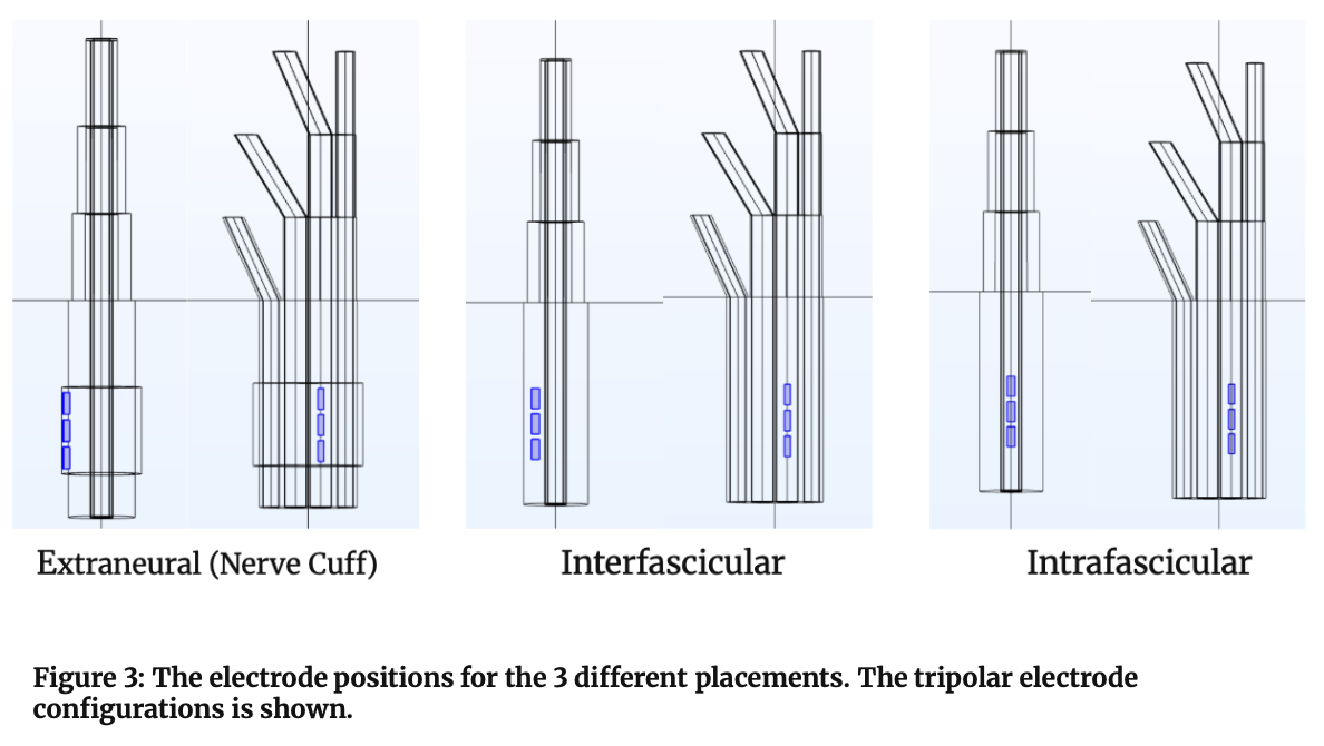
From there, the electrodes themselves were created. They were modelled as small 3D patches and placed in their appropriate locations for the nine different test conditions. In our model, the 3rd fascicle was treated as the primary sensory fascicle, and therefore the electrodes were all lined up on this specific fascicle so there can be an even comparison between the conditions. Figure 3 shows the tripolar configuration for each of the three different positions. For the given configurations, the monopole has one anode at $+1\,\mathrm{mA}$; the dipole has one cathode at $-1\,\mathrm{mA}$ and one anode at $+1\,\mathrm{mA}$; the tripolar has one cathode at $-1\,\mathrm{mA}$ and two anodes at $+0.5\,\mathrm{mA}$ each.

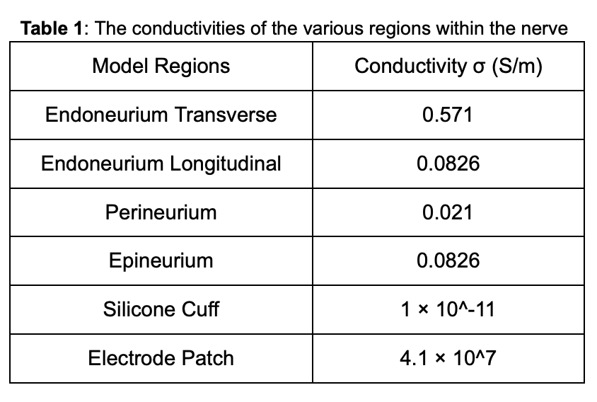
Once all proper segmentation and graphics were completed, the material conductivities and permeabilities were assigned. The endoneurium exhibited both transverse and longitudinal conductivities of $0.571\,\mathrm{S/m}$ and $0.0826\,\mathrm{S/m}$, respectively. Thus, the endoneurium was anisotropic with less resistance to current flow longitudinally than transversely. The perineurium had an isotropic $0.021\,\mathrm{S/m}$ electrical conductivity, serving as a resistive layer, and the epineurium had an isotropic conductivity of $0.0826\,\mathrm{S/m}$. Additionally, the nerve cuff was modelled as silicone with a conductivity of $1 \times 10^{-11}\,\mathrm{S/m}$, and the electrode patch was composed of gold with a conductivity of $4.1 \times 10^{7}\,\mathrm{S/m}$. These values can all be seen in Table 1 (Kinouchi et al., 1997). Regarding assumptions, the model assumes uniform tissue properties within each layer, no temperature rise, no electrochemical reactions, and perfect-conductor electrodes. A free tetrahedral mesh was used to discretize the electrode–tissue interface, and a boundary-layer mesh was also placed within the perineurial entities. Additionally, the PARDISO direct solver was used with a zero initial potential and standard tolerances under stationary conditions. Lastly, the “solve” button was utilized to calculate the voltages over space. From there, a 3D “cut-line” was inserted into each of 4 fascicles, which spatially sampled a voltage vs. arc-length position trace. These four traces for each of the 9 test conditions could then be fed into NEURON.

Methods: NEURON Model

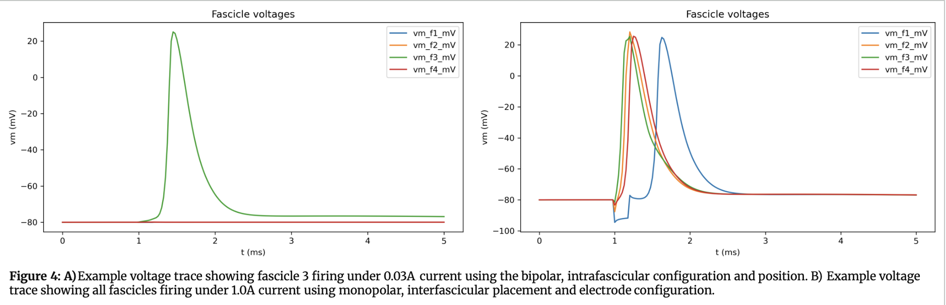
We simulated peripheral nerve activation in NEURON using the McIntyre–Richardson–Grill (MRG) myelinated axon model. The model consists of 21 nodes of Ranvier connected by paranodal (MYSA/FLUT) and internodal (STIN) segments, with diameter-specific electrical properties tuned for mammalian myelinated fibers at $37\,^{\circ}\mathrm{C}$ (McIntyre et al., 2002). Each segment includes an extracellular mechanism, allowing externally applied fields to be imposed directly. In COMSOL, as aforementioned, voltage profiles were obtained using “cut-lines” that characterize the voltage distribution along each fascicle. We interpolated each fascicle’s COMSOL arc-length profile onto every segment center of the MRG axon, using a linear scale map by default. The spatially mapped, unit-voltage profile is multiplied by a rectangular pulse (delay $1\,\mathrm{ms}$, width $0.2\,\mathrm{ms}$, and scaled by amplitude) to form per-segment extracellular time-series in $\mathrm{mV}$ (Fig. 4). That scale is multiplied by the unit spatial profile to form per-segment extracellular voltages. We then called NEURON’s Vector.play() function, which attaches each segment’s time series to its extracellular potential. Finally, we ran the simulation using a timestep of $0.025\,\mathrm{ms}$ for $5\,\mathrm{ms}$. We recorded transmembrane voltage ($V_m$) at the central node to quantify activation.

Methods: Selectivity Analysis

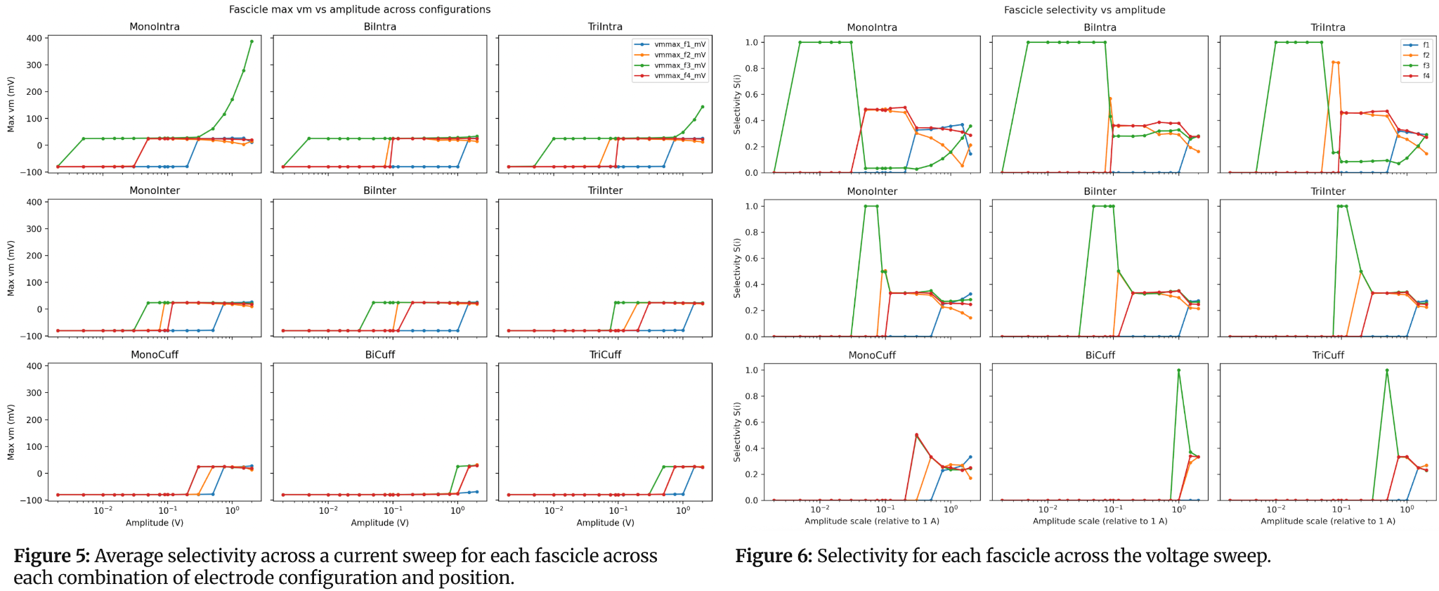
Amplitude sweeps — time-series obtained by titrating amplitudes from $5\times 10^{-5}$ to $2$ times the input current of $1\,\mathrm{mA}$ — were applied to each electrode configuration/position to obtain the threshold for fascicle activation. For each sweep, the peak $V_m$ for each fascicle was determined at every amplitude scale (Fig. 5), and normalized by dividing by that fascicle’s own maximum over all amplitudes in the sweep to get a normalized maximum voltage $V_i$ for each fascicle (Eq. 1). Selectivity at each amplitude was then computed from the normalized voltage values (Eq. 2, Fig. 6) (Yoo et al., 2004). Finally, selectivity was averaged across the sweep for each fascicle in each configuration, enabling direct comparison (e.g., fascicle 3) across all conditions.

$$V_{i,\mathrm{norm}} = \frac{V_i}{\max V_i} \tag{1}$$ $$S_i = \frac{V_{i,\mathrm{norm}}}{\sum_j V_{j,\mathrm{norm}}} \tag{2}$$

Statistical Analysis

To determine which stimulation configuration has the highest average selectivity for fascicle three across the current sweeps, we employed an approximate mixed-effects approach. We used an ordinary least squares model with categorical fixed effects for configuration and amplitude. We estimated marginal means per configuration averaged over the observed amplitude distribution, and used pairwise configuration contrasts with Holm-adjusted $p$-values. This allowed us to assess the statistical significance ($p < 0.05$) of differences between stimulation configurations/electrode placements for each fascicle.

Results

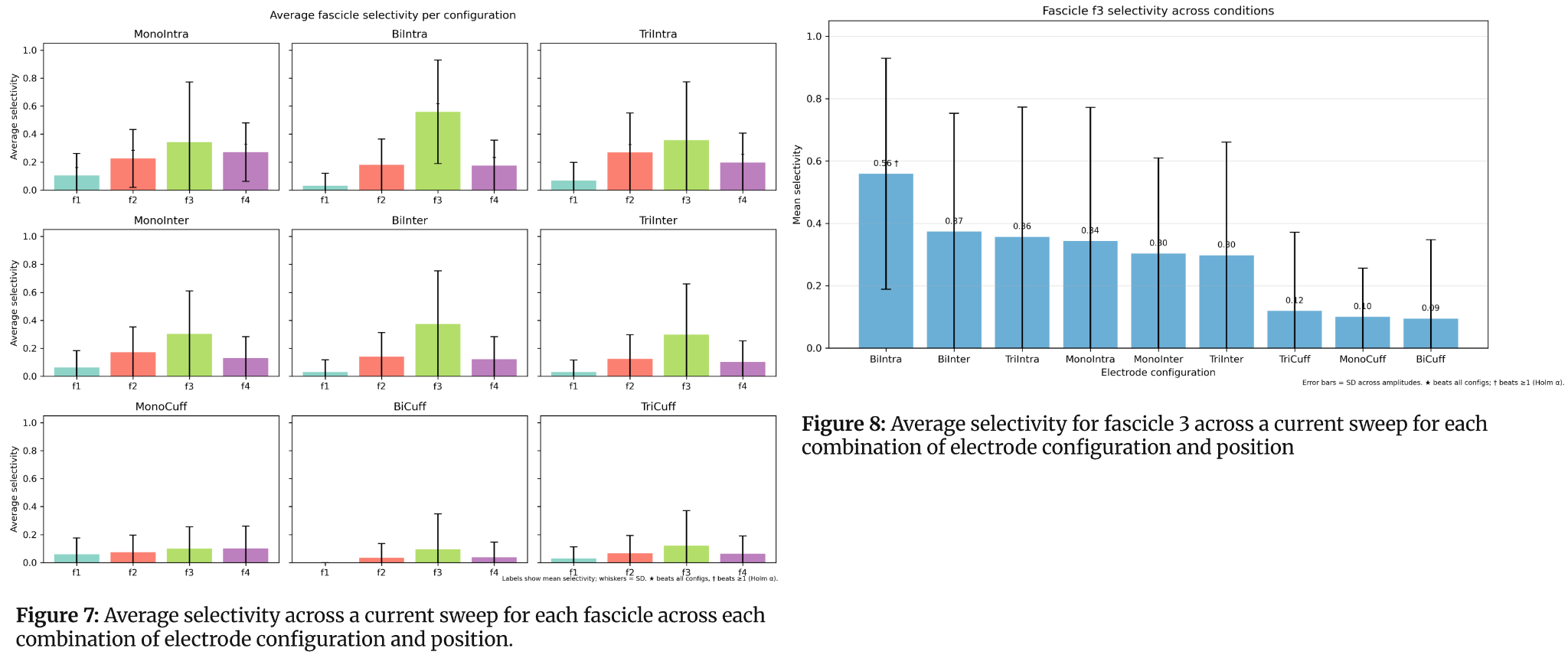
For fascicle 3 — the sensory fascicle — the bipolar intrafascicular configuration was the most favorable ($0.419 \pm 0.060$). The bipolar intrafascicular configuration beats the bipolar cuff, the monopolar cuff, and the tripolar cuff. The estimated marginal means (mean selectivity $\pm$ standard error across the current sweep) favored the monopolar intrafascicular configuration/placement for fascicle 1 ($0.078 \pm 0.012$), and the monopolar intrafascicular configuration significantly exceeded bipolar cuff, bipolar interfascicular, bipolar intrafascicular, tripolar cuff, and tripolar interfascicular. For fascicle 2, the tripolar intrafascicular configuration was favored ($0.201 \pm 0.026$). The tripolar intrafascicular configuration beats the bipolar cuff, the tripolar cuff, and the monopolar cuff configurations, while the monopolar intrafascicular beats the bipolar cuff and the tripolar cuff. For fascicle 4, the monopolar intrafascicular configuration was the best, beating the bipolar cuff, the bipolar intrafascicular, the monopolar cuff, the monopolar interfascicular, the tripolar cuff, and the tripolar interfascicular. Additionally, the tripolar intrafascicular and bipolar intrafascicular configurations beat the bipolar cuff (Fig. 7–8).

Conclusion and Discussion

In this study, we evaluated how electrode placement (extraneural, interfascicular, and intrafascicular) and configuration (monopolar, bipolar, and tripolar) influence selectivity during sensory fascicle stimulation. By using a COMSOL 3D model of the ulnar nerve and the MRG myelinated axon model in NEURON, we could directly compare all 9 possibilities.

Across electrode placement conditions, the intrafascicular case consistently showed the highest selectivity, highlighting the importance of minimizing the electrode–axon distance and confining current spread to prevent neighboring fascicles from being stimulated. Among these cases, the intrafascicular bipolar stimulation was the most selective configuration for fascicle 3 — the target sensory fascicle for sensory restoration in amputees — as it had the highest mean selectivity across the amplitude sweep. This finding showed that the bipolar intrafascicular conditions had an effective balance between spatial focusing of the electric field and efficient depolarization of targeted axons.

Theoretically, while a tripolar configuration should offer the best current confinement, as our hypothesis stated, its performance in our study was largely inconsistent with our original hypothesis. This electrode configuration required higher effective amplitudes, which suggested over-constraint of the field within small intrafascicular volumes. Additionally, the monopolar configuration cases experienced poorer selectivity due to broader current spread, as theory suggests. Despite differences between theoretical/experimental results and limitations in our assumptions, integrating COMSOL-derived potentials with NEURON-based activation analysis provided a robust framework for quantitatively comparing stimulation strategies.

Overall, while we did not find that a single configuration/position combination statistically beat out all other combinations, this study provides strong computational evidence that bipolar intrafascicular stimulation is promising for the most selective stimulation of a fascicle for sensory restoration, particularly for upper-limb neuroprosthetic applications such as those involving the ulnar nerve. Future work will improve biophysical realism, incorporate efficiency metrics alongside selectivity, and add additional geometries/pulse parameters to the analysis. Cumulatively, such efforts can guide next-generation peripheral nerve stimulation that minimizes off-target activation and power requirements, while maximizing functional specificity.

References

[1] Becker, Rachel E. and Biagio Manna. “Anatomy, Shoulder and Upper Limb, Ulnar Nerve.” StatPearls, StatPearls Publishing, 24 July 2023.

[2] Kinouchi, Y. et al. “Fast in vivo measurements of local tissue impedances using needle electrodes.” Medical & Biological Engineering & Computing 35.5 (1997): 486–92. doi:10.1007/BF02525528

[3] McIntyre, Cameron C. et al. “Modeling the excitability of mammalian nerve fibers: influence of afterpotentials on the recovery cycle.” Journal of Neurophysiology 87.2 (2002): 995–1006. doi:10.1152/jn.00353.2001

[4] Yoo, Paul B. et al. “Selective stimulation of the canine hypoglossal nerve using a multi-contact cuff electrode.” Annals of Biomedical Engineering 32.4 (2004): 511–9. doi:10.1023/b:abme.0000019170.74375.fb