Sequential Change-Point Detection for Chronic Neural Interfaces using Adaptive Thresholds Under an Electrode Degradation Model

Abbreviations

Introduction

Background and Motivation

Drug-resistant temporal lobe epilepsy (TLE) affects roughly one-third of the 50 million people worldwide living with epilepsy [1]. The NeuroPace responsive neurostimulation (RNS) system is the current clinical standard; however, it monitors only two anatomical targets via eight contact electrode arrays, with stimulation latencies exceeding 1 second [2,3]. TLE seizures are network-scale events with onset in the hippocampus and propagation through the amygdala, thalamus, and temporal cortex within seconds. Since the seizure onset time is unknown a priori, the detection problem can be framed as a quickest change-point detection problem, as described by Wald [4], Lorden [5], and Shiryaev [6].

Stochasticity is present across all levels: seizure onset time can be modeled as a random variable (RV); local field potential (LFP) recordings are ridden with Brownian-motion-type noise with long-term shifts in variance and attenuation in signal-to-noise ratio due to immune response and glial encapsulation of electrodes [7]; and seizure propagation delays across network nodes are RVs drawn from patient-specific anatomy and connectivity. A stochastic framework for data processing is thus required. Prior work has demonstrated that cumulative-sum (CUSUM)-based seizure detectors can outperform fixed-window classifiers for both scalp and intracranial EEG recordings in terms of detection latency, while maintaining comparable false-positive rates, motivating a deeper look into sequential methods and their robustness to the chronic signal degradation inherent in implanted interfaces [8, 9].

This project provides (1) a chronic degradation model capturing both signal attenuation and noise increases, (2) Monte Carlo validation of analytically derived performance bounds for three sequential detectors, and (3) a 6-month simulation to compare both fixed and adaptive thresholds.

Central Hypothesis

I hypothesize that adaptive-threshold sequential change-point detectors (SPRT, CUSUM, Shiryaev–Roberts), applied to a hidden Markov observation model of seizure dynamics with Gaussian diffusion observations, will maintain clinically viable detection performance over a simulated six-month chronic period despite impedance-driven SNR degradation from glial encapsulation, whereas fixed-threshold detectors will exhibit measurable deterioration in both detection delay and false positive rate over the same period.

Mathematical Background

The Log-Likelihood Ratio

Most sequential detection procedures monitor a constant stream of observations and, stepwise, ask whether the distribution has changed. The standard feature used as evidence is the log-likelihood ratio (LLR). Given a sequence of observations $E_1, E_2, \ldots$ drawn independently from one of two distributions, under the null hypothesis $H_0$ each observation has density $f_0$, and under $H_1$ each has density $f_1$. The log-likelihood ratio for any one observation is thus:

$$\lambda_n = \log\left(\frac{f_1(E_n)}{f_0(E_n)}\right) \tag{1}$$

This ratio is positive when $E_n$ is more likely under $H_1$ than under $H_0$, and negative otherwise. For this study, given a shift in the mean $\theta$, the Gaussian distributions that result are $H_0 \sim \mathcal{N}(0,\sigma^2)$ and $H_1 \sim \mathcal{N}(\theta,\sigma^2)$ for $\theta > 0$. In this case, the LLR reduces to:

$$\lambda_n = \frac{\theta}{\sigma^2} E_n - \frac{\theta^2}{2\sigma^2} \tag{2}$$

Here, the first term is directly proportional to the observation, so large values of $E_n$ provide stronger evidence for $H_1$. The second term accounts for the size of the shift. Under $H_0$, the expected increment is $\mathbb{E}_0[\lambda_n] = -\theta^2/(2\sigma^2) < 0$, so the accumulated evidence drifts toward $H_0$. Under $H_1$, the sign is reversed and the LLR drifts toward $H_1$.

When the variances differ between the hypotheses, $H_0 \sim \mathcal{N}(0,\sigma_0^2)$ versus $H_1 \sim \mathcal{N}(\theta,\sigma_1^2)$, the LLR becomes:

$$\lambda_n = \log\frac{\sigma_0}{\sigma_1} - \frac{(E_n-\theta)^2}{2\sigma_1^2} + \frac{E_n^2}{2\sigma_0^2} \tag{3}$$

This is quadratically related to $E_n$ (unlike the equal-variance case).

The Sequential Probability Ratio Test

Wald’s Sequential Probability Ratio Test (SPRT) [4] accumulates the LLR over time and stops when a boundary is reached:

$$\Lambda_N = \sum_{n=1}^{N} \lambda_n, \qquad T = \inf\{N : \Lambda_N \notin (A,B)\} \tag{4}$$

where $A < 0 < B$. If $\Lambda_N > B$, decide $H_1$; if $\Lambda_N < A$, decide $H_0$. In this study, when $H_0$ is declared the SPRT is reset and rerun continuously.

Per Wald, with false-positive probability $\alpha$ and false-negative probability $\beta$:

$$A \approx \log\frac{\beta}{1-\alpha}, \qquad B \approx \log\frac{1-\beta}{\alpha} \tag{5}$$

For $\alpha = \beta = 0.01$, this yields $A = -4.6$ and $B = 4.6$. Expected sample sizes under each hypothesis are:

$$\mathbb{E}_0[T] \approx \frac{(1-\alpha)A + \alpha B}{\mathbb{E}_0[\lambda]}, \qquad \mathbb{E}_1[T] \approx \frac{(1-\beta)B + \beta A}{\mathbb{E}_1[\lambda]} \tag{6}$$

Cumulative Sum

SPRT assumes the distribution lies at either $H_0$ or $H_1$ from the start. For seizure detection, the distribution starts at $H_0$ and transitions to $H_1$ at an unknown time $\nu$. Page’s CUSUM [2] discards evidence favoring $H_0$:

$$W_n = \max(0,\, W_{n-1} + \lambda_n), \quad W_0 = 0 \tag{7}$$ $$T = \inf\{n : W_n > h\} \quad\text{for a threshold } h > 0 \tag{8}$$

The detection delay under $H_1$ is approximately:

$$\mathbb{E}_1[\mathrm{delay}] \approx \frac{h}{\mathbb{E}_1[\lambda]} \tag{9}$$

and the average run length under $H_0$ satisfies an exponential bound of the form

$$\mathrm{ARL}_0 \approx \frac{e^{\zeta h}}{\zeta\,\mathbb{E}_0[\lambda e^{\zeta\lambda}]} \tag{10}$$

where $\zeta$ is the positive root of $\mathbb{E}_0[e^{\zeta\lambda}] = 1$ (for equal variances, $\zeta = 1$).

The Shiryaev–Roberts Procedure

The Shiryaev–Roberts (SR) procedure [7, 11] aggregates evidence that a change occurred at some past time:

$$R_n = \sum_{k=1}^{n} \prod_{j=k}^{n} \frac{f_1(E_j)}{f_0(E_j)} \tag{11}$$

or recursively:

$$R_n = \left(1 + R_{n-1}\right)\frac{f_1(E_n)}{f_0(E_n)}, \quad R_0 = 0 \tag{12}$$

with stopping time

$$T = \inf\{n : R_n > A\} \quad\text{for a threshold } A. \tag{13}$$

The Pareto Frontier

For a sequential detection procedure, a trade-off exists between detection delay and false-positive rate. By sweeping detector thresholds and plotting operating points, relative efficiency can be compared. The Pareto frontier is the set of points at which no procedure achieves both shorter delay and lower false-positive rate.

Methods

State Process and Observation Model

The seizure state is modeled as a continuous-time process $X(t)\in\{0,1\}$ where $X=0$ is interictal and $X=1$ is ictal. The change point $\nu$ is the transition time from 0 to 1. Features used to compute the LLR are high-gamma band energy (70–150 Hz), computed across 100-ms windows at 10 Hz. The feature-level observation model is:

$$E_n \;\big|\; X = \begin{cases} \mathcal{N}(0,\sigma_0^2) & X=0 \\ \mathcal{N}(\theta,\sigma_1^2) & X=1 \end{cases} \tag{14}$$

where $\theta>0$ is the change in expected high-gamma activity at seizure onset, $\sigma_0$ is the interictal noise standard deviation, and $\sigma_1$ is the ictal noise standard deviation. The ratio $r=\sigma_1/\sigma_0$ is a model parameter (default $r=1.5$), swept over $r\in\{1.0,1.2,1.5,2.0\}$.

Dual Chronic Degradation Model

Glial scar encapsulation attenuates the recorded signal and raises the noise floor [7, 10]:

$$\theta(t) = \theta_0\bigl(1 - \beta(1 - e^{-t/\tau_g})\bigr) \tag{15}$$ $$\sigma_0(t) = \sigma_{0,\mathrm{init}}\bigl(1 + \alpha(1 - e^{-t/\tau_g})\bigr) \tag{16}$$

with $\sigma_1(t)=r\,\sigma_0(t)$. Default parameters: $\alpha=0.75$, $\beta=0.2$, $\tau_g=2.5$ months, $r=1.5$.

Combined SNR Trajectory

$$\mathrm{SNR}(t) = \frac{\theta(t)}{\sigma_0(t)} = \frac{\theta_0\bigl(1-\beta(1-e^{-t/\tau_g})\bigr)}{\sigma_{0,\mathrm{init}}\bigl(1+\alpha(1-e^{-t/\tau_g})\bigr)} \tag{17}$$

At month 6 with the parameters above, $\theta(6)\approx 0.82\,\theta_0$ and $\sigma_0(6)\approx 1.68\,\sigma_{0,\mathrm{init}}$, giving $\mathrm{SNR}(6)\approx 0.49\,\mathrm{SNR}(0)$.

Detector Implementation and Adaptive Estimation

The three algorithms follow the recursions in Eqs. 4, 7–8, and 12–13 on LLR sequences from Eq. 3. Adaptive detectors track $\sigma_0$ and $\theta$ with two-timescale exponential moving averages and recalibrate thresholds daily (SPRT via Eq. 5; CUSUM/SR via target ARL$_0$/delay). Monte Carlo evaluation uses 10,000 trials per acute condition and 100 six-month chronic simulations across nine algorithm $\times$ threshold-mode combinations (fixed, adaptive-slow, adaptive-fast), plus robustness checks with Student-$t$ noise and variance-ratio sweeps.

Results

Observation Model and Degradation Dynamics

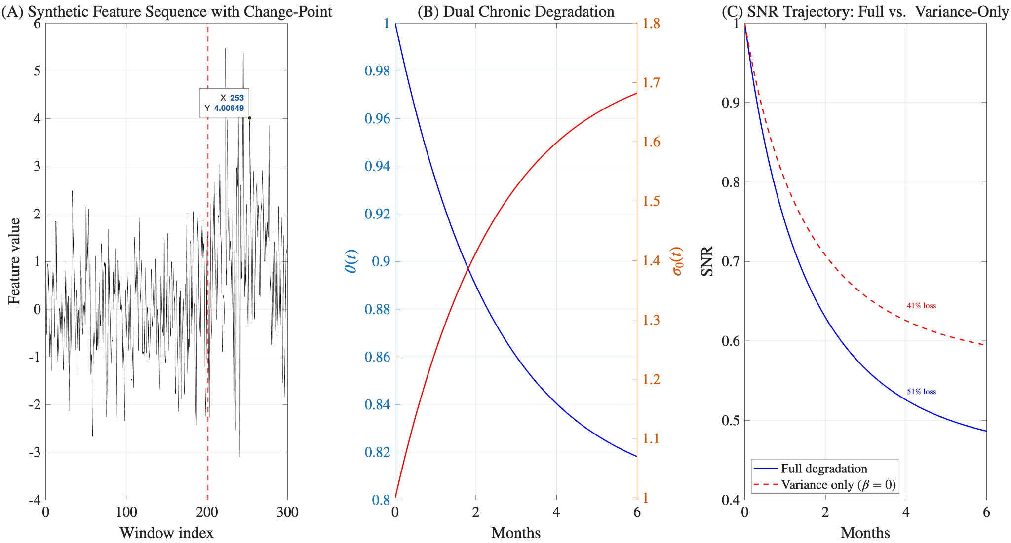
The full degradation model predicts a 51% drop in SNR after 6 months post-implantation vs a 41% drop for the model that only included variance degradation. This is due to the exclusion of the signal amplitude attenuation in the latter model. The majority of the degradation occurs during the first three months and is driven by $\tau_g = 2.5$ months (Fig. 1).

Detector Behavior on a Single Trial

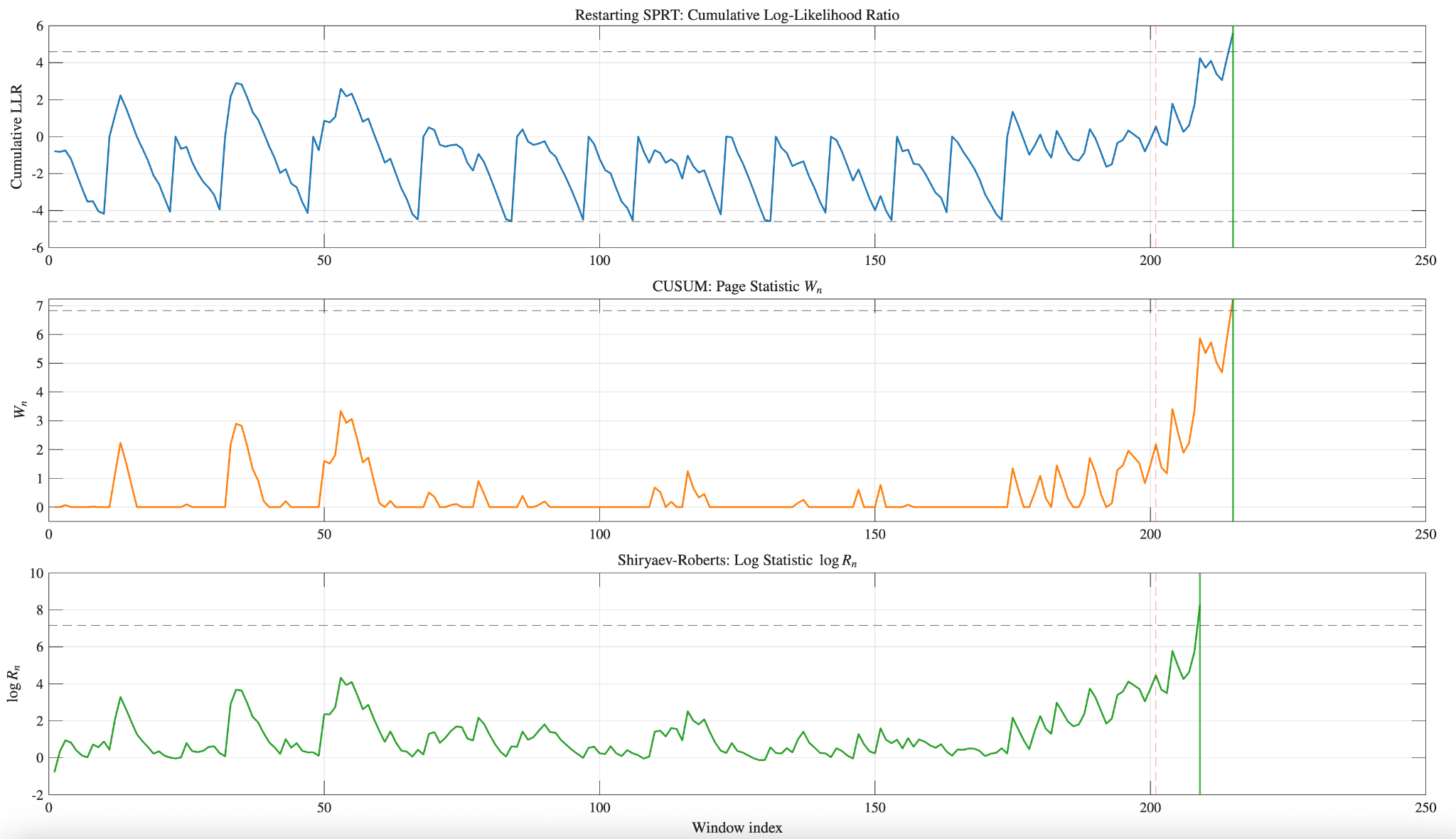
All three detectors detect within 10–15 windows of the change point (1–1.5 seconds at 10 Hz). The SPRT demonstrates restarting behavior during the interictal period when boundary $A$ is reached. The CUSUM statistic remains near 0 during the interictal period due to the max operator. The SR statistic reflects interictal variation by incorporating possible past change points. After the change point, all three statistics show a positive drift and cross the detection boundaries.

Pareto Frontier

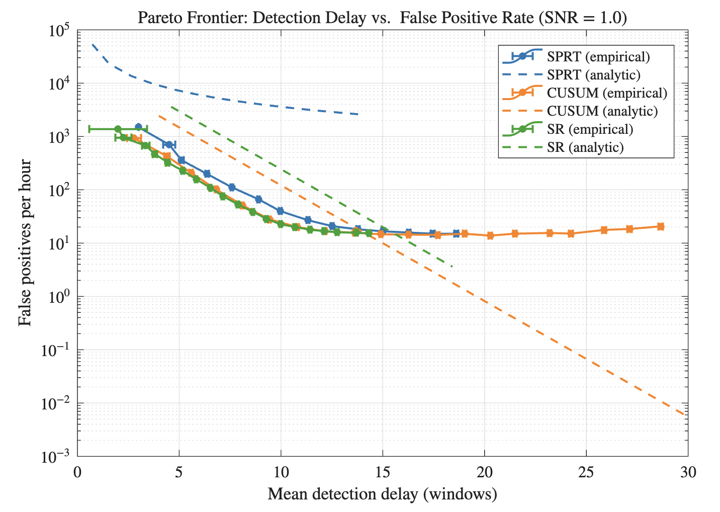
CUSUM and SR algorithms have shorter detection delays than SPRT at similar false positive rates. The CUSUM and SR empirical plots overlap substantially, whereas SPRT has a higher average false-positive rate for a given detection delay. Analytic predictions align with empirical trends for CUSUM and SR at smaller mean detection delays; the SPRT analytical prediction overestimates the false positive rate but matches the overall trend.

Analytic Validation Across SNR

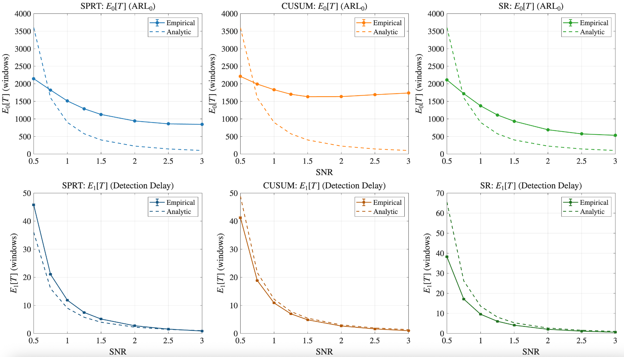
All three detectors show monotonic behavior. Both $\mathrm{ARL}_0$ and detection delay decrease as SNR increases. Detection of $H_1$ occurs much faster than the average stopping time under $H_0$, as expected.

Chronic Detection Delay

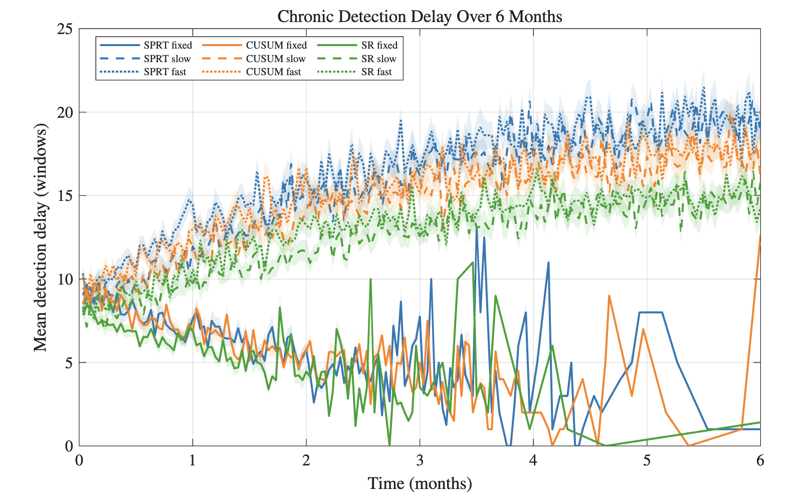
Adaptive threshold detectors show clear but modest performance degradation over the six-month simulation (Figure 5). The SPRT exhibits the most severe deterioration, with mean delay increasing from approximately 8 windows at month 0 to approximately 21 windows by month 6. CUSUM and SR degrade less, from approximately 7 to 15 windows. Fixed thresholds demonstrate a steady decrease in detection delay as degradation increases false positives.

Chronic False Positive Rate

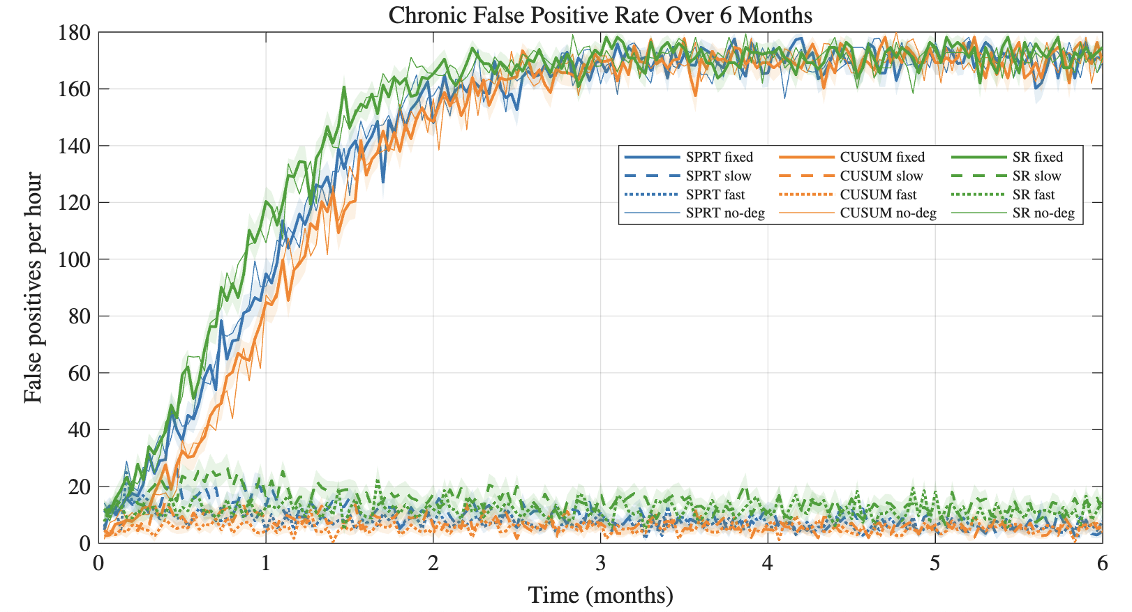
The fixed-threshold algorithms exhibit a severe increase in the false positive rate, from $<20$ false positives per hour to over 160 by month 2–3 (Fig. 6)—clinically unusable. Adaptive threshold models hover below 20 false positives per hour. This separation is the strongest evidence supporting the central hypothesis, alongside the modest delay increase in Fig. 5.

Adaptive Parameter Tracking

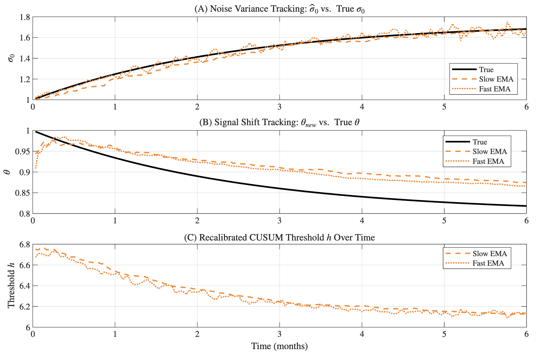
The two-timescale EMA estimation procedure can track the evolution of parameters (Fig. 7). Adaptive-fast and adaptive-slow models track the shift in variance; signal-shift estimates show greater discrepancy and tend to overestimate $\theta$. The recalibrated CUSUM threshold $h$ decreases over six months as parameters drift.

Sensitivity Analysis

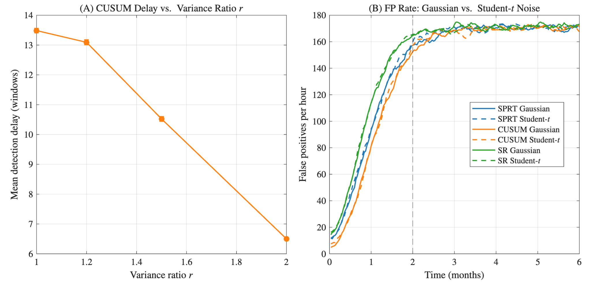
As expected, detection delay decreases as $r$ increases from 1.0 to 2.0. Gaussian and Student-$t$ noise produce very similar false-positive rates under chronic drift, confirming that parameter drift dominates the noise-distribution choice for the conditions tested.

Conclusion

The central hypothesis predicted that adaptive-threshold detectors would outperform fixed-threshold detectors over the 6-month degradation period. The simulations confirm this: fixed-threshold detectors show decreasing mean detection delay only because false-positive rates explode, whereas adaptive detectors accept a modest delay increase of about 5–10 windows ($0.5$–$1$ second) while holding false-positive rates steady. CUSUM and SR outperform SPRT on the Pareto frontier and in chronic simulation; SPRT degrades fastest because its restarting mechanism is more sensitive to miscalibration. Among CUSUM and SR, performance is nearly identical, with CUSUM offering a slightly more practical implementation.

This study shows that quickest-detection algorithms applied to synthetic seizure features retain clinical utility under adaptive thresholds across a 6-month chronic degradation model. Future work may examine fusion across distributed recording nodes for closed-loop stimulation that better matches the network architecture of TLE.

AI Disclosure

I used Claude (Anthropic) to implement simulation infrastructure: the Monte Carlo engine, batch feature generation, figure formatting, and file I/O. I also used it for debugging code and vectorizing inner loops. All mathematical derivations were performed by hand, including the log-likelihood ratios, SPRT threshold algebra, CUSUM ARL$_0$ bound, and the miscalibrated-drift analysis motivating adaptive detection. The detector algorithms and analytic bounds were coded from these derivations. Simulation design, analysis, interpretation, and all prose are my own work.

References

[1] Asadi-Pooya, A. A., Stewart, G. R., Abrams, D. J., & Sharan, A. (2017). Prevalence and Incidence of Drug-Resistant Mesial Temporal Lobe Epilepsy in the United States. World Neurosurgery, 99, 662–666.

[2] Nair, D. R. et al. (2020). Nine-year prospective efficacy and safety of brain-responsive neurostimulation for focal epilepsy. Neurology, 95(9), e1244–e1256.

[3] Fisher, R. et al. (2010). Electrical stimulation of the anterior nucleus of the thalamus for treatment of refractory epilepsy. Epilepsia, 51(5), 899–908.

[4] Wald, A. (1945). Sequential tests of statistical hypotheses. Annals of Mathematical Statistics, 16(2), 117–186.

[5] Lorden, G. (1971). Procedures for reacting to a change in distribution. Annals of Mathematical Statistics, 42(6), 1897–1908.

[6] Shiryaev, A. N. (1963). On optimum methods in quickest detection problems. Theory of Probability & Its Applications, 8(1), 22–46.

[7] Polikov, V. S. et al. (2005). Response of brain tissue to chronically implanted neural electrodes. Journal of Neuroscience Methods, 148(1), 1–18.

[8] Zandi, A. S. et al. (2010). Automated real-time epileptic seizure detection in scalp EEG recordings using an algorithm based on wavelet packet transform. IEEE Transactions on Biomedical Engineering, 57(7), 1639–1651.

[9] Osorio, I. et al. (2002). Performance reassessment of a real-time seizure-detection algorithm on long ECoG series. Epilepsia, 43(12), 1522–1535.

[10] Salatino, J. W. et al. (2017). Glial responses to implanted electrodes in the brain. Nature Biomedical Engineering, 1, 862–877.

[11] Pollak, M. (1985). Optimal detection of a change in distribution. Annals of Statistics, 13(1), 206–227.

[12] Tartakovsky, A., Nikiforov, I., & Basseville, M. (2014). Sequential Analysis: Hypothesis Testing and Changepoint Detection. CRC Press.